This chapter introduces one of the simplest yet very useful types of machine learning algorithms: linear models. First, a theory for the basic linear model algorithm will be laid down. Then, the employment of regularization to generate other common types of linear model algorithms, e.g., Ridge and Lasso, will be explained. Linear models are, by nature, proposed for regression. The extension of such algorithms to classification, including both binary classification and multiclass classification, will be introduced next. Finally, we will show the use of kernel functions to turn linear models into nonlinear methods for regression and classification.

It is worthwhile to clarify some common confusing points before we start the journey.
First, "linear model" or "linear models" here refers to the algorithm(s) that helps us obtain the actual models. As explained in previous chapters, algorithms are methods to obtain models, while models are algorithms that have been instantiated or fixed with model parameters, which are determined by specific datasets during training. In a simple way, an algorithm can be analogous to the use of a polynomial function to fit a dataset, while a model is the polynomial with parameters fixed in this curve fitting process. But it is kind of a convention to call such algorithms "linear model" or "linear models" in machine learning. This convention is still kept here to stay aligned with most machine learning literature.

Second, in a narrow sense, linear model as a machine learning topic contains only those linear model algorithms in which the independent variables (representing the data attributes), e.g., $x_i,x_2,\cdots ,x_i,\cdots$$x_i,x_2,\cdots ,x_i,\cdots$x_(i),x_(2),cdots,x_(i),cdotsx_{i}, x_{2}, \cdots, x_{i}, \cdots$x_i,x_2,\cdots ,x_i,\cdots$ in $\overrightarrow{x}$$\overrightarrow{x}$vec(x)\vec{x}$\overrightarrow{x}$, maintain a linear relationship. That is, the dependent variable (representing the label) $y$$y$yy$y$ is a linear combination of these independent variables $x_i$$x_i$x_(i)x_{i}$x_i$. However, it is quite common to adopt kernel functions to give linear models nonlinear capacities. Thus, the linear models with the use of kernel functions are still introduced as part of the linear model topic in a broad sense in this book.

Third, there are big overlaps between linear model, linear regression, and curve fitting with linear functions, and they may even refer to the same thing in some cases. This confusion is caused by the fact that these terms are proposed and used by people from different disciplines, e.g., computer science, math, and engineering. In this book, the use of linear models is mostly inherited from machine learning and data analysis, thus it focuses on the use of linear models for addressing regression and classification problems. In this context, an analytical solution can be obtained directly due to the intentional confinement to simple linear models. By contrast, relevant topics like curve fitting (especially nonlinear curve learning), which may require the use of complicated math functions and optimization techniques to iteratively obtain the optimal solution, will not be discussed here.

The idea of linear models is to use a linear mathematical function of one or more variables to approach some given function value(s) of these variable(s). In machine learning, such a function value correspond to the label of a sample, while such variables correspond to different attributes of the sample. Frequently, in the context of math functions, independent variables and dependent variables are used to refer to the sample attributes and labels, respectively. In some cases, especially when the context of statistics and probability is adopted, it is also common to see the use of predictors and response variables.

Let us first outline a typical problem for linear models using the math language. In the simple case, let us only consider one variable $x$$x$xx$x$. Then, the function $f(x)$$f(x)$f(x)f(x)$f(x)$ can be formulated as

where $[x,y]$$[x,y]$[x,y][x, y]$[x,y]$ represents one data point in a space consisting of 2 axes (or dimensions) and $\cdot$$\cdot$*\cdot$\cdot$ is the (arithmetic) product between two scalars.

In a regression problem, there are usually multiple data points in this space, e.g., $I$$I$II$I$ points $[(x_1,y_1),(x_2,y_2),\cdots ,(x_I,y_I)]$$\left[\left(x_1,y_1\right),\left(x_2,y_2\right),\cdots ,\left(x_I,y_I\right)\right]$[(x_(1),y_(1)),(x_(2),y_(2)),cdots,(x_(I),y_(I))]\left[\left(x_{1}, y_{1}\right),\left(x_{2}, y_{2}\right), \cdots,\left(x_{I}, y_{I}\right)\right]$[(x_1,y_1),(x_2,y_2),\cdots ,(x_I,y_I)]$, which are the "measurements" that need to be approximated with Eq. 4.1. The goal of using a linear model for regression is to find the function $f(x)=w\cdot x+b$$f(x)=w\cdot x+b$f(x)=w*x+bf(x)=w \cdot x+b$f(x)=w\cdot x+b$ closest to all the measurements. The closest curve can be associated with the smallest total distance between the measured values $y_i$$y_i$y_(i)y_{i}$y_i$ and predicted values $f\left(x_i\right)$$f\left(x_i\right)$f(x_(i))f\left(x_{i}\right)$f\left(x_i\right)$. Usually, the Euclidean distance is selected as the measure of distance in regression tasks. Under this condition, a regression task using a linear model can be mathematically described as

where $w^{\ast }$$w^{\ast }$w^(**)w^{*}$w^{\ast }$ and $b^{\ast }$$b^{\ast }$b^(**)b^{*}$b^{\ast }$ are the optimal model parameters $w$$w$ww$w$ and $b$$b$bb$b$, and $\arg \underset{(w,b)}{min}$$\arg \underset{(w,b)}{min}$arg min_((w,b))\arg \min _{(w, b)}$\arg \underset{(w,b)}{min}$ means to minimize a function parameterized by $w$$w$ww$w$ and $b$$b$bb$b$. This equation presents a formulation of linear regression with the ordinary least squares.

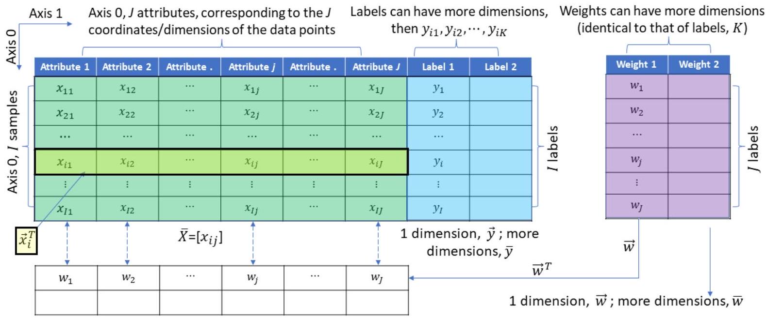
The data in general regression applications can be much more complicated than that in the above simple case. In particular, each data sample may contain more than one attribute, which can be viewed as multiple random variables from a statistics perspective. We can understand the typical data that we will deal with in linear model applications using a data structure that is compatible with those adopted in tools like NumPy and Pandas.

Figure 4.1: Illustration of general data structure
As shown in Fig. 4.1, the unlabeled data $\overline{X}$$\overline{X}$bar(X)\bar{X}$\overline{X}$ has $I$$I$II$I$ samples (rows), and each sample ${\overrightarrow{x}}_i^T$${\overrightarrow{x}}_i^T$vec(x)_(i)^(T)\vec{x}_{i}^{T}${\overrightarrow{x}}_i^T$ consists of $J$$J$JJ$J$ attributes (columns). In fact, any sample in its original shape, ${\overrightarrow{x}}_i$${\overrightarrow{x}}_i$vec(x)_(i)\vec{x}_{i}${\overrightarrow{x}}_i$, is essentially a column vector as follows,

and all the unlabeled data form $\overline{X}={[{\overrightarrow{x_1}}^T,{\overrightarrow{x_2}}^T,\cdots ,{\overrightarrow{x_I}}^T]}^T$$\overline{X}={\left[{\overrightarrow{x_1}}^T,{\overrightarrow{x_2}}^T,\cdots ,{\overrightarrow{x_I}}^T\right]}^T$bar(X)=[ vec(x_(1))^(T), vec(x_(2))^(T),cdots, vec(x_(I))^(T)]^(T)\bar{X}=\left[{\overrightarrow{x_{1}}}^{T},{\overrightarrow{x_{2}}}^{T}, \cdots,{\overrightarrow{x_{I}}}^{T}\right]^{T}$\overline{X}={[{\overrightarrow{x_1}}^T,{\overrightarrow{x_2}}^T,\cdots ,{\overrightarrow{x_I}}^T]}^T$ (or written as $\overline{X}=[{\overrightarrow{x_1}}^T;{\overrightarrow{x_2}}^T;\cdots ;{\overrightarrow{x_I}}^T]$$\overline{X}=\left[{\overrightarrow{x_1}}^T;{\overrightarrow{x_2}}^T;\cdots ;{\overrightarrow{x_I}}^T\right]$bar(X)=[ vec(x_(1))^(T); vec(x_(2))^(T);cdots; vec(x_(I))^(T)]\bar{X}=\left[{\overrightarrow{x_{1}}}^{T} ;{\overrightarrow{x_{2}}}^{T} ; \cdots ;{\overrightarrow{x_{I}}}^{T}\right]$\overline{X}=[{\overrightarrow{x_1}}^T;{\overrightarrow{x_2}}^T;\cdots ;{\overrightarrow{x_I}}^T]$ ). Note that each sample $i$$i$ii$i$ in Fig. 4.1 is ${\overrightarrow{x}}_i^T$${\overrightarrow{x}}_i^T$vec(x)_(i)^(T)\vec{x}_{i}^{T}${\overrightarrow{x}}_i^T$ (a row) instead of $\overrightarrow{x_i}$$\overrightarrow{x_i}$vec(x_(i))\overrightarrow{x_{i}}$\overrightarrow{x_i}$ (a column). This data structure and tensor notation (a hybrid notation, explained in the book Appendices) are adopted throughout this book.

For any sample, ${\overrightarrow{x}}_i$${\overrightarrow{x}}_i$vec(x)_(i)\vec{x}_{i}${\overrightarrow{x}}_i$, the linear function of the variables, ${\overrightarrow{x}}_{ij}(j\in \{1,\cdots ,J\})$${\overrightarrow{x}}_{ij}(j\in \{1,\cdots ,J\})$vec(x)_(ij)(j in{1,cdots,J})\vec{x}_{i j}(j \in\{1, \cdots, J\})${\overrightarrow{x}}_{ij}(j\in \{1,\cdots ,J\})$, can be formulated as the following linear combination:

where ${[x_{i1},x_{i2},\cdots ,x_{iJ},y_i]}^T$${\left[x_{i1},x_{i2},\cdots ,x_{iJ},y_i\right]}^T$[x_(i1),x_(i2),cdots,x_(iJ),y_(i)]^(T)\left[x_{i 1}, x_{i 2}, \cdots, x_{i J}, y_{i}\right]^{T}${[x_{i1},x_{i2},\cdots ,x_{iJ},y_i]}^T$ represents one labeled data point in a space consisting of $J+1$$J+1$J+1J+1$J+1$ axes, in which $J$$J$JJ$J$ axes represent the $J$$J$JJ$J$ variables while the remaining axis represents the label. In some places, people consider the label separately and thus state the data has $J$$J$JJ$J$ dimensions. $f\left({\overrightarrow{x}}_i\right)$$f\left({\overrightarrow{x}}_i\right)$f( vec(x)_(i))f\left(\vec{x}_{i}\right)$f\left({\overrightarrow{x}}_i\right)$ is still used to map the input $\overline{X}$$\overline{X}$bar(X)\bar{X}$\overline{X}$ to the output $\overrightarrow{y}$$\overrightarrow{y}$vec(y)\vec{y}$\overrightarrow{y}$. The meaning of the ', , sign changes from the multiplication in arithmetic to dot product in tensor algebra as the variables change from scalars $x_i$$x_i$x_(i)x_{i}$x_i$ 's to vectors $\overrightarrow{x}{}_i$$\overrightarrow{x}{}_i$vec(x)_(i)\vec{x}{ }_{i}$\overrightarrow{x}{}_i$ 's.

In a regression problem, usually, multiple points, e.g., $I$$I$II$I$ points in this case, are available as "measurements". The goal of using a linear model for regression is to find a function (e.g., a curve in 2 D ), $f(\overrightarrow{x})={\overrightarrow{w}}^T\cdot \overrightarrow{x}+b$$f(\overrightarrow{x})={\overrightarrow{w}}^T\cdot \overrightarrow{x}+b$f( vec(x))= vec(w)^(T)* vec(x)+bf(\vec{x})=\vec{w}^{T} \cdot \vec{x}+b$f(\overrightarrow{x})={\overrightarrow{w}}^T\cdot \overrightarrow{x}+b$, that is the closest to all the measurements. Again, the closest curve is usually associated with the smallest total distance between the measurement points and the curve, which is usually formulated using the Euclidean distance. Under this condition, the regression task using a linear model can be mathematically described as

The linear model can be written using arrays as

The above equation can be reformulated as

where,

The loss function (cost function or objective function) can be written as

The use of the sign "." can be confusing: this sign can refer to either scalar product (regular multiplication between scalars) or dot product. As introduced in the previous chapters, concepts like vectors and tensors are widely used in engineering, and sometimes, the tensor notation can be more convenient than the index notation, which is widely used in traditional machine learning. For example, algorithms formulated using the tensor notation can be more easily expressed using the tensor notation without worrying about the operations between tensors if the operators are clearly defined. Also, tensors can be more straightforwardly related to the arrays used in coding and computing. Thus, the tensor notation is adopted with minor modifications in most places of this book, including the majority of this chapter. More information about notation and operations can be found in Chapter 1 and the appendices at the end of the book.

To facilitate the use of tensors and the tensor notation, it is clarified that scalars are viewed as 0th order tensors, vectors is 1 st order tensors, while 2 nd and higher order tensors, which are called tensors in a narrow sense, are termed tensors or high-order tensors. Also, as for operators or operation signs, in this book, when '. ' is used between a scalar and any other tensors (scalars, vectors or high-order tensors), it is used for scalar product: the product between the scalar and the other scalar or elements in the tensors; when it is used between a vector and another 1st or higher order tensors, it refers to a dot (vector) product or equivalently a tensor product with a single contraction. In Python coding, '*' is used for the former type of product (scalar product), while '@' is used for the latter (dot product). Following this rule will make the implementation of the theories in this book much simpler than what can be seen in other literature.

Then, the mathematical description of the regression problem using a linear model is

The following closed-form solution to the above equation can be obtained:

The following Python code presents the construction of a linear model based on the above theory. This model was created with very a dataset consisting of eight data points, each of which has two attributes. Random noise was added to the dataset.

import numpy as np
              import matplotlib.pyplot as plt
              from mpl_toolkits import mplot3d
              # Create data
              X_list = [[1.,1.],[1.,2.],[2.,2.],[2.,3.],[1.5,2.5],[2.,4.],[1.,3.],[3.,1.5]] # Create unlabeled
                data point/instance using a Python list
              X = np.array(X_list) # Turn instance into a NumPy array
              Proj = np.array([1,2]) # Create perfect labels
              y = np.dot(X,Proj)+3 # Add intercept
              y = y + np.random.rand(y.size) # Add noise to mimic experimental measurements
              # Define a function to perform analytical solution to linear model problems
              def LinearRegression(X,y):
                X_bar = np.hstack((X,np.ones([X.shape[0],1]))) # I = 8 by J+1 = 3
                W_hat = np.linalg.inv(X_bar.T @ X_bar) @ X_bar.T @ y # J+1 = 3 by 1
                return W_hat, X_bar
              # Symbols are the same as those in the textbook
              W_hat, X_bar= LinearRegression(X,y)
              W = W_hat [:-2]
              b = W_hat[-2:]
              # Solution
              Y_fit = np.dot(X_bar,W_hat)
              # Plot and compare results
              fig = plt.figure()
              ax = plt.axes(projection='3d')
              ax.scatter(X[:,0],X[:, 1],y,'b*')
              ax.scatter(X[:,0],X[:,1],Y_fit,'rd')
              

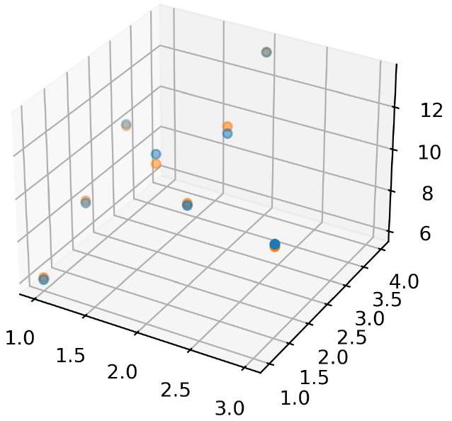
The original data points and data points predicted with the trained model are plotted in .

Figure 4.2: Training result of a linear model

When the number of samples $(I)$$(I)$(I)(I)$(I)$ is relatively small and the number of features $(J)$$(J)$(J)(J)$(J)$ is relatively large, basic linear models such as the above one with the ordinary least squares are susceptible to overfitting issues. To avoid or prevent overfitting, we can resort to several methods. One typical method is to reduce the number of features. For this purpose, significant features will be retained while some insignificant ones will be abandoned. Another popular method for avoiding overfitting in linear models is regularization. The goal of regularization is to obtain models with both high accuracy and low complexity. The addition of a regularization term to the above basic linear model can generate some other popular linear models such as Ridge, Lasso, and elastic net regression models. In the following, information for Ridge and Lasso linear models will be presented.

The Ridge regression is a linear model with $L_2$$L_2$L_(2)L_{2}$L_2$ norm regularization [43]. With a regularization term, the loss function of Ridge is usually constructed as follows,

Then, the Ridge regression problem can be formulated as

where $\lambda {\hat{w}}^T\cdot \hat{w}=\lambda \sum _{i=1}^J{\hat{w}}_i^2$$\lambda {\widehat{w}}^T\cdot \widehat{w}=\lambda \sum _{i=1}^J {\widehat{w}}_i^2$lambda hat(w)^(T)* hat(w)=lambdasum_(i=1)^(J) hat(w)_(i)^(2)\lambda \hat{w}^{T} \cdot \hat{w}=\lambda \sum_{i=1}^{J} \hat{w}_{i}^{2}$\lambda {\hat{w}}^T\cdot \hat{w}=\lambda \sum _{i=1}^J{\hat{w}}_i^2$.
The closed-form solution to the above Ridge regression problem can be derived as

where $\overline{I}$$\overline{I}$bar(I)\bar{I}$\overline{I}$ is a identify matrix with dimensions of $(J+1)$$(J+1)$(J+1)(J+1)$(J+1)$ by $(J+1)$$(J+1)$(J+1)(J+1)$(J+1)$.
In addition to the closed-form solution, we can also use the gradient descent method to solve the above optimization problem associated with the Rigid regression. The gradient of the loss function, which is a key in such optimization solution processes, is given below,