Previous
Association Rule Learning
Contents
Table of Contents
Next
Gradient-Based RL

Chapter 15

Value-Based Reinforcement Learning

15.1. Overview

This chapter presents the basics of Reinforcement Learning (RL) and, based on that, introduces value-based RL as one of the two major categories of RL algorithms. For this goal, the basic RL concepts, including Markov Decision Process and essential RL terms, like environment, state, action, value, reward and policy, will be explained first. Next we will have an RL demonstration using simple virtual environments. Then, the Bellman equation, which casts the basis for the "learning" or improvement of an RL learning agent, will be discussed. This includes the Bellman equation's mathematical formulations, deduction, and use. After going through the basics, we will start the introduction to value-based RL algorithms with an overview of popular RL algorithms. Following that, typical value-based RL algorithms including two time-difference algorithms, i.e., Q-learning and Sarsa, and one episode-update algorithm, i.e., Monte Carlo, will be introduced. Details will be provided to cover both theories and guidelines for the implementation of these algorithms.

15.2. Basics of Reinforcement Learning

15.2.1. Basic Concepts

In a loose sense, any learning problem can be conceptualized as the interaction between a learning agent and the world whereby the agent performs learning and application of the learned knowledge. In supervised and unsupervised learning, all the data, no matter whether labeled or unlabeled, is ready and carries knowledge about the world. By contrast, data in reinforcement learning is not available before a learning process starts. Instead, the agent obtains the data as the learning agent interacts with the environment. The data can be understood as "labeled" because we need to figure out what to do (described as "action" in RL; can be viewed as labels) under what conditions (described as "state" in reinforcement learning; can be viewed as data without labels). The model will be continuously improved as more data is obtained in the training process. The model's performance also needs to be evaluated with metrics in reinforcement learning. Such metrics are so-called reward functions that tell the goodness of specific actions for certain states.
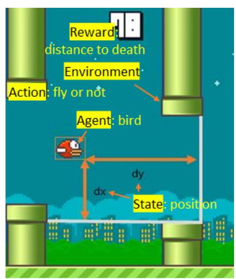
Based on the above introduction, we can generally conceptualize reinforcement learning as illustrated in Fig. 15.1. The world outside of a learning agent is modeled as an environment. In this flappy bird game, the agent is the bird or the player controlling the agent, and the environment is the space consisting of the pipe obstacles. In order to describe the learning process, we need to know the current status of the learning agent, i.e., state, and the action the learning agent will take to interact with the environment. In this example, the state is the location of the bird, while the action is to fly or not. The action may bring the agent to a different (new) state and get reward from the environment that leads to beneficial results, e.g., survive longer in the game. The goal of any reinforcement learning process is to maximize the rewards so that the learning agent can gain a better performance. The Markov Decision Process (MDP) to be introduced will present a more strict model for conceptualizing such sequential decision processes [153, 154].

15.2.2. Markov Decision Process

The studies of MDP stemmed from the realm of optimal control. In 1957, a U.S. researcher, Richard Bellman [155] first proposed the discrete time MDP via an optimal control model. Between 1960 and 1962, Howard [156] and Blackwell [157] proposed a dynamic programming algorithm for solving MDP problems. The MDP and its solution methods
Figure 15.1: Example of environment and its elements in reinforcement learning
were later adopted for applications in various areas, such as autonomous control, suggestion systems, and reinforcement learning. In addition to the above essential components like state, action, and reward, MDP is characterized by the Markov property: the state at the current time is only related to the state and action at the previous time and independent of the state and action at other time points. This can be described using the following probability equation:
(15.1) P [ s t + 1 s t ] = P [ s t + 1 s 1 , a 1 , s 2 , a 2 , s t ] (15.1) P s t + 1 s t = P s t + 1 s 1 , a 1 , s 2 , a 2 , s t {:(15.1)P[s_(t+1)∣s_(t)]=P[s_(t+1)∣s_(1),a_(1),s_(2),a_(2)cdots,s_(t)]:}\begin{equation*} P\left[s_{t+1} \mid s_{t}\right]=P\left[s_{t+1} \mid s_{1}, a_{1}, s_{2}, a_{2} \cdots, s_{t}\right] \tag{15.1} \end{equation*}(15.1)P[st+1st]=P[st+1s1,a1,s2,a2,st]
This equation means that the consideration of earlier states does not make a difference in MDP.
Sequential decision problems based on MDP can be grouped into two categories: model-based and model-free. Dynamic programming was proposed for model-based problems. That is, the influence of the learning agent's action on the environment - the probability P s s a P s s a P_(ss^('))^(a)P_{s s^{\prime}}^{a}Pssa and reward r s s a r s s a r_(ss^('))^(a)r_{s s^{\prime}}^{a}rssa of entering a new state, s s s^(')s^{\prime}s, after taking an action, a a aaa, in the current state, s s sss - is known. By contrast, reinforcement learning was proposed for model-free problems, but it can also be used to solve model-based problems. More information about the classification of RL algorithms, including model-based and modelfree categories in a broad sense, will be presented before we start working on the first major category of RL algorithms, i.e., value-based RL algorithms, in this chapter.
The Bellman equation is viewed as the core of dynamic programming. Based on it, a solution to MDP problems can be derived. Because both dynamic programming and reinforcement learning are intended for sequential decision problems, they share many concepts in common including the Bellman equation. Due to this reason, many people also perceive the Bellman equation as the core of reinforcement learning. However, reinforcement learning usually includes additional materials in addition to the sole use of the Bellman equation.

15.2.3. Policy Function, State Function, State-Action Function, and Reward Function

A policy determines how an agent selects an action in a state of the environment. This policy can be deterministic, that is, one action will be selected in a specific state. Or, the policy can also be stochastic, that is, in a specific state, the agent can select an action from different candidate actions (discrete or continuous) with different probabilities. In RL, it can be more specifically referred to as the learning policy, while in applications like control tasks, it may be called the control policy. Every policy can be formulated using a policy function:
(15.2) π ( s ) : S A (15.2) π ( s ) : S A {:(15.2)pi(s):S|->A:}\begin{equation*} \pi(s): S \mapsto A \tag{15.2} \end{equation*}(15.2)π(s):SA
With the above equation, when a state, s s sss, is entered as the input, the policy function will give out an action, a a aaa, as the output.
Value functions, in a broad sense, contain both V V VVV and Q Q QQQ. But in a narrow sense, we call V V VVV a value function and Q Q QQQ an action-value function. Both V V VVV and Q Q QQQ are widely used in RL algorithms. These two functions are closely related, and they can be converted to each other. Thus, in some RL algorithms, such as Q-learning and Sarsa, you may only see one of them, such as Q Q QQQ. These two functions can be confusing. Some aspects of these two types of functions are clarified here.
First, both of the two functions are usually associated with a specific learning policy. For example, we write them as V π ( s ) V π ( s ) V^(pi)(s)V^{\pi}(s)Vπ(s) and Q π ( s , a ) Q π ( s , a ) Q^(pi)(s,a)Q^{\pi}(s, a)Qπ(s,a), where the superscript π π pi\piπ marks the policy. However, in algorithms such as Q-learning and Sarsa,
the policy is continuously improved as more data is processed by the agent to improve the policy. Thus, π π pi\piπ may also be omitted to avoid confusion.
Second, from the symbol, we can see that, V ( s ) V ( s ) V(s)V(s)V(s) is the value of a state (without mentioning any specific action), while Q ( s , a ) Q ( s , a ) Q(s,a)Q(s, a)Q(s,a) is the value associated with an action in a state, in which both an action and a state are needed. These two types of functions can be defined as follows. V π ( s ) V π ( s ) V^(pi)(s)V^{\pi}(s)Vπ(s) is the expected value of rewards following policy π π pi\piπ forever when the agent starts the learning process from the state s : V π ( s ) = E ( R ) s : V π ( s ) = E ( R ) s:V^(pi)(s)=E(R)s: V^{\pi}(s)=\mathbb{E}(R)s:Vπ(s)=E(R). Mathematically, this is formulated as
(15.3) V π ( s , π ) = E π ( R s , π ) = E π [ k = 0 γ k r t + k + 1 s 0 = s ] (15.3) V π ( s , π ) = E π ( R s , π ) = E π k = 0 γ k r t + k + 1 s 0 = s {:(15.3)V^(pi)(s","pi)=E_(pi)(R∣s","pi)=E_(pi)[sum_(k=0)^(oo)gamma^(k)r_(t+k+1)∣s_(0)=s]:}\begin{equation*} V^{\pi}(s, \pi)=\mathbb{E}_{\pi}(R \mid s, \pi)=\mathbb{E}_{\pi}\left[\sum_{k=0}^{\infty} \gamma^{k} r_{t+k+1} \mid s_{0}=s\right] \tag{15.3} \end{equation*}(15.3)Vπ(s,π)=Eπ(Rs,π)=Eπ[k=0γkrt+k+1s0=s]
where R R RRR is the long-term reward. R R RRR at the current step t t ttt can be obtained by summing up the rewards at different steps as R t = k = 0 γ k r t + k + 1 R t = k = 0 γ k r t + k + 1 R_(t)=sum_(k=0)^(oo)gamma^(k)r_(t+k+1)R_{t}=\sum_{k=0}^{\infty} \gamma^{k} r_{t+k+1}Rt=k=0γkrt+k+1. This equation can also be written as
(15.4) V π ( s , π ) = E π ( R t s , π ) = E π [ k = 0 γ k r t + k + 1 s t = s ] (15.4) V π ( s , π ) = E π R t s , π = E π k = 0 γ k r t + k + 1 s t = s {:(15.4)V^(pi)(s","pi)=E_(pi)(R_(t)∣s,pi)=E_(pi)[sum_(k=0)^(oo)gamma^(k)r_(t+k+1)∣s_(t)=s]:}\begin{equation*} V^{\pi}(s, \pi)=\mathbb{E}_{\pi}\left(R_{t} \mid s, \pi\right)=\mathbb{E}_{\pi}\left[\sum_{k=0}^{\infty} \gamma^{k} r_{t+k+1} \mid s_{t}=s\right] \tag{15.4} \end{equation*}(15.4)Vπ(s,π)=Eπ(Rts,π)=Eπ[k=0γkrt+k+1st=s]
By contrast, Q π ( s , a ) Q π ( s , a ) Q_(pi)(s,a)Q_{\pi}(s, a)Qπ(s,a) is the expected value of rewards yielded by first taking action a a aaa in state s s sss and then following the policy π π pi\piπ forever. Therefore, Q Q QQQ can be related to rewards as
(15.5) Q π ( s , π ) = E ( R s , a , π ) (15.5) Q π ( s , π ) = E ( R s , a , π ) {:(15.5)Q^(pi)(s","pi)=E(R∣s","a","pi):}\begin{equation*} Q^{\pi}(s, \pi)=\mathbb{E}(R \mid s, a, \pi) \tag{15.5} \end{equation*}(15.5)Qπ(s,π)=E(Rs,a,π)
Based on the definition, the two types of functions can be converted to each other using the following equations.
V π ( s ) = E a [ Q π ( s , a ) ] (15.6a) = a π ( a s ) Q π ( s , a ) (15.6b) Q π ( s , a ) = s P s s a [ r s s a + γ V π ( s ) ] V π ( s ) = E a Q π ( s , a ) (15.6a) = a π ( a s ) Q π ( s , a ) (15.6b) Q π ( s , a ) = s P s s a r s s a + γ V π s {:[V^(pi)(s)=E_(a)[Q^(pi)(s,a)]],[(15.6a)=sum_(a)pi(a∣s)Q^(pi)(s","a)],[(15.6b)Q^(pi)(s","a)=sum_(s^('))P_(ss^('))^(a)[r_(ss^('))^(a)+gammaV^(pi)(s^('))]]:}\begin{align*} V^{\pi}(s) & =\mathbb{E}_{a}\left[Q^{\pi}(s, a)\right] \\ & =\sum_{a} \pi(a \mid s) Q^{\pi}(s, a) \tag{15.6a}\\ Q^{\pi}(s, a)= & \sum_{s^{\prime}} P_{s s^{\prime}}^{a}\left[r_{s s^{\prime}}^{a}+\gamma V^{\pi}\left(s^{\prime}\right)\right] \tag{15.6b} \end{align*}Vπ(s)=Ea[Qπ(s,a)](15.6a)=aπ(as)Qπ(s,a)(15.6b)Qπ(s,a)=sPssa[rssa+γVπ(s)]
where π ( a s ) π ( a s ) pi(a∣s)\pi(a \mid s)π(as) is the probability of selecting action a a aaa if we follow policy π π pi\piπ (policy can be determinate but here a more general definition with indeterminate policy is adopted), P s s a P s s a P_(ss^('))^(a)P_{s s^{\prime}}^{a}Pssa is the probability of moving from state s s sss to s s s^(')s^{\prime}s if we take action a , r s s a a , r s s a a,r_(ss^('))^(a)a, r_{s s^{\prime}}^{a}a,rssa is the reward gained as we move from s s sss to s s s^(')s^{\prime}s. In Q-learning and Sarsa, random factors were added via ϵ ϵ epsilon\epsilonϵ-greedy, which corresponds to P s s a P s s a P_(ss^('))^(a)P_{s s^{\prime}}^{a}Pssa. In the literature, we can also see r s a = s P s s a r s s a r s a = s P s s a r s s a r_(s)^(a)=sum_(s^('))P_(ss^('))^(a)r_(ss^('))^(a)r_{s}^{a}=\sum_{s^{\prime}} P_{s s^{\prime}}^{a} r_{s s^{\prime}}^{a}rsa=sPssarssa.
It is also common to use * to represent the optimal policy, which leads to the highest long-term reward. Accordingly, V ( s ) V ( s ) V^(**)(s)V^{*}(s)V(s) is the maximum possible value of V π ( s ) V π ( s ) V^(pi)(s)V^{\pi}(s)Vπ(s) :
(15.7) V ( s ) = max π V π ( s ) (15.7) V ( s ) = max π V π ( s ) {:(15.7)V^(**)(s)=max_(pi)V^(pi)(s):}\begin{equation*} V^{*}(s)=\max _{\pi} V^{\pi}(s) \tag{15.7} \end{equation*}(15.7)V(s)=maxπVπ(s)
The theory of MDP states that if π π pi^(**)\pi^{*}π is an optimal policy, we will act optimally. Therefore, we will take the optimal action by choosing the action from Q ( s , ) Q ( s , ) Q^(**)(s,*)Q^{*}(s, \cdot)Q(s,), and this generates the optimal V ( s ) V ( s ) V^(**)(s)V^{*}(s)V(s) :
(15.8) V ( s ) = max a Q ( s , a ) (15.8) V ( s ) = max a Q ( s , a ) {:(15.8)V^(**)(s)=max_(a)Q^(**)(s","a):}\begin{equation*} V^{*}(s)=\max _{a} Q^{*}(s, a) \tag{15.8} \end{equation*}(15.8)V(s)=maxaQ(s,a)
It is worthwhile to point out that, in policy-based algorithms, we usually evaluate the policy, i.e., π ( a s ) π ( a s ) pi(a∣s)\pi(a \mid s)π(as), which can be viewed as a probability distribution of actions. By contrast, in value-based algorithms, we usually use and improve the optimal functions V V V^(**)V^{*}V or/and Q Q Q^(**)Q^{*}Q, which can be viewed as V V VVV or/and Q Q QQQ values that can best help us identify the optimal action (e.g., action a a aaa with the highest Q ( s , a ) Q ( s , a ) Q(s,a)Q(s, a)Q(s,a) value in s s sss ).

15.2.4. Implementation of RL Environment

In this section, brief information is provided to show how to work with an RL environment. Two different ways will be illustrated. The first way involves the use of environments created by RL packages such as OpenAI Gym [158]. OpenAI Gym provides functions for users to easily employ a variety of RL environments. These environments can be used to test RL algorithms that are developed by the users, so that the user can focus on the RL algorithms instead of wasting time to find, implement, or calibrate RL environments. The second refers to the development of RL environments from scratch.

Implementation with OpenAI Gym

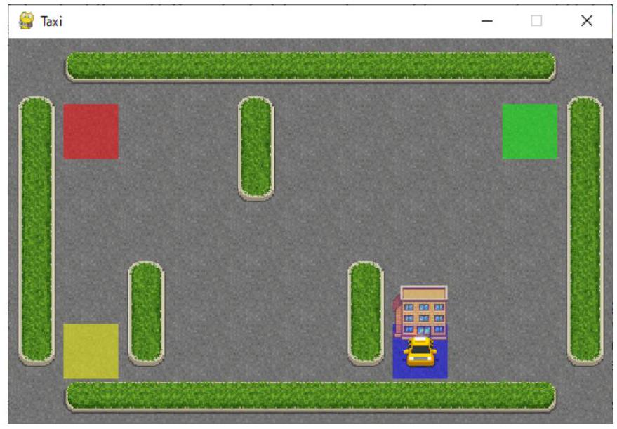
We use an environment called "Taxi-v3" from OpenAI Gym as an example. As illustrated in Fig. 15.2, the taxi needs to start at a random location, pick up and drop off a passenger at two locations randomly selected from the four special locations marked with four colors. There are six actions: 0 : move south, 1 : move north, 2 : move east, 3: move west, 4 : pickup passenger, and 5: drop off passenger. The map has 25 cells ( 5 rows by 5 columns). Therefore, there are 500 states: 5 rows 5 5 **5* 55 columns 5 5 **5* 55 passenger positions (at four special locations + in taxi) 4 4 **4* 44 destinations = 500 = 500 =500=500=500 states.
Figure 15.2: Drawing of Taxi-v3 environment in Open Gym
The following code shows the use and check of the environment. The first step to use this environment is to import the package and initialize the environment using "gym.make('Taxi-v3')". We can also check or/and use the size of the action and state spaces to get a better understanding of the environment. Such information will also likely be needed in later use of the environment for RL.
import numpy as np
              import gymnasium as gym # Old versions use "import gym"
              # Initialization
              env = gym.make("Taxi-v3", render_mode="human") # Call the "Taxi-v3" environment from gym with the
                name "env"
              action_size = env.action_space.n # Obtain the size of the action space: how many actions. There are
                six here
              state_size = env.observation_space.n # Obtain the size of the state space: 5 rows * 5 columns * 5
                passenger positions * 4 destinations =500 states
              
A key step in the use of such RL environment is to make one step in an episode. In this step, a new state will be obtained. Also, a reward value will be obtained after taking the action. Another variable is the signal to indicate whether the episode ends. In OpenAI Gym, this signal is represented using a variable called "done". This can be seen in the following code.
# Update state
                state_new, reward, done, _, _ = env.step(action)
              
When an episode is finished, i.e., some conditions for ending the episode are met, we usually need to stop the RL iterations. This can be done as follows.
# Stop an episode when the environment tells an episode ends
                if done == 1:
                    print('This is the #%i training episode' % n)
                    break
              
After each episode or before we start testing, we will need to reset the environment. In testing, we also need to use loops by iteratively calling the "env.step()" function to add more steps within each episode. In addition, an "env.render()" function is provided in OpenAI Gym to illustrate the results. This is shown in the following code.
# Testing
              state = env.reset()[0]
              while True:
                # Choose an action based on the Q table only
                action = np.argmax(Table[state]) # Choose an action based on the Q table
                state, reward, done, _, _ = env.step(action)
                env.render() # Green is passenger; Red is destination
                if done == 1:
                    break
              

Implementation from Scratch

In this part, the construction of a very simple environment that can be used in a way similar to OpenAI Gym environments is illustrated in the following code. Because the code for building the environment serves as Python functions that can be imported by other Python code, we used object-oriented programming to develop the code. The code includes a few key parts similar to OpenAI Gym: initialize variables and functions, develop functions to reset the environment, develop a function to make one step in the episode (including assigning rewards and stopping the episode), and develop a render function to illustrate the state when using the episode.
import numpy as np
              class treasure1D:
                def ___init__(self,N):
                    self.n_cell = N # The greater this number, the higher n_episode is needed
                    self.Reward = np.zeros(self.n_cell);
                    self.Reward[-1]=1.0 # n_cell cells, only the rightmost has reward (end of game)
                    self.States = range(self.n_cell)
                    self.state = np.random.choice(self.States)
                    self.reward = 0
                    self.done = False
                    self.observation_size = 1 # Number of elements in observation (there is only one in this env
                : state/position)
                def reset(self):
                    self.state = np.random.choice(self.States)
                    self.reward = 0
                    self.done = False
                    return self.state
                def step(self,action):
                    # Update state
                    reward = 0
                    if action == 'left' or action == 0:
                        if self.state == self.States[0]: # Leftmost
                            state_new = self.state # Does not move
                            self.done = True
                            self.reward = -10
                        else:
                            state_new = self.state - 1 # Obtain new state s^prime
                    else:
                        if self.state == self.States[-1]: # rightmost
                            state_new = self.state # Does not move
                            self.done = True
                            self.reward = 10
                        else:
                            state_new = self.state + 1 # Obtain new state s^prime
                    self.state = state_new
                    return self.state, self.reward, self.done, []
                def render(self):
                    print ("The state is ", self.state, "The reward is ",self.reward)
              
This environment simulates a very simple 1D treasure hunt game. In each episode, an agent will be placed at a random cell of a 1D map consisting of multiple cells. The agent needs to find the treasure in the rightmost cell. Rewards/penalties are only assigned to the cells on the two ends of the map. The agent cannot move out of the map from the left. Thus, it
will stay in the leftmost cell when it tries to move left from there, and a reward of -10 (penalty of 10 ) is applied when that happens. An episode ends when the agent reaches the rightmost cell, i.e., finding the treasure, and a reward of 10 is made.

15.3. Bellman Equation

The Bellman equation lays out a relationship between the state value function or the action-state value function in the current state and that in the following state. Therefore, this equation appears in a recursive format and can be used iteratively to obtain V V VVV or/and Q Q QQQ in an episode. In this subsection, we will first give out the Bellman equation in different forms. Then, details will be offered to show how the Bellman equation in typical forms can be derived to understand the essence of learning in RL.

15.3.1. Formulations of Bellman Equation

The Bellman equation can be formulated with the state value function and the action-state value function. The Bellman equation formulated with the state value function describes the values function in the current state s s sss and the value function in the following state s s s^(')s^{\prime}s :
(15.9) V π ( s ) = a π ( a s ) Q π ( s , a ) = a π ( a s ) s P s s a [ r s s a + γ V π ( s ) ] (15.9) V π ( s ) = a π ( a s ) Q π ( s , a ) = a π ( a s ) s P s s a r s s a + γ V π s {:(15.9)V^(pi)(s)=sum_(a)pi(a∣s)Q^(pi)(s","a)=sum_(a)pi(a∣s)sum_(s^('))P_(ss^('))^(a)[r_(ss^('))^(a)+gammaV^(pi)(s^('))]:}\begin{equation*} V^{\pi}(s)=\sum_{a} \pi(a \mid s) Q^{\pi}(s, a)=\sum_{a} \pi(a \mid s) \sum_{s^{\prime}} P_{s s^{\prime}}^{a}\left[r_{s s^{\prime}}^{a}+\gamma V^{\pi}\left(s^{\prime}\right)\right] \tag{15.9} \end{equation*}(15.9)Vπ(s)=aπ(as)Qπ(s,a)=aπ(as)sPssa[rssa+γVπ(s)]
Likewise, the Bellman equation formulated with the action-state value function describes the action-state value function in the current state s s sss and that in the following state s s s^(')s^{\prime}s
(15.10) Q π ( s , a ) = s P s s a [ r s s a + γ V π ( s ) ] = s P s s a [ r s s a + γ a π ( a s ) Q π ( s , a ) ] (15.10) Q π ( s , a ) = s P s s a r s s a + γ V π s = s P s s a r s s a + γ a π a s Q π s , a {:(15.10)Q^(pi)(s","a)=sum_(s^('))P_(ss^('))^(a)[r_(ss^('))^(a)+gammaV^(pi)(s^('))]=sum_(s^('))P_(ss^('))^(a)[r_(ss^('))^(a)+gammasum_(a^('))pi(a^(')∣s^('))Q^(pi)(s^('),a^('))]:}\begin{equation*} Q^{\pi}(s, a)=\sum_{s^{\prime}} P_{s s^{\prime}}^{a}\left[r_{s s^{\prime}}^{a}+\gamma V^{\pi}\left(s^{\prime}\right)\right]=\sum_{s^{\prime}} P_{s s^{\prime}}^{a}\left[r_{s s^{\prime}}^{a}+\gamma \sum_{a^{\prime}} \pi\left(a^{\prime} \mid s^{\prime}\right) Q^{\pi}\left(s^{\prime}, a^{\prime}\right)\right] \tag{15.10} \end{equation*}(15.10)Qπ(s,a)=sPssa[rssa+γVπ(s)]=sPssa[rssa+γaπ(as)Qπ(s,a)]
Based on the above equations and the relationship in Section 15.2.3, we can obtain the following Bellman equation for the optimal state value function and action-state value function:
(15.11a) V ( s ) = max a Q ( s , a ) = max a s P s s a [ r s s a + γ V π ( s ) ] . (15.11b) Q ( s , a ) = s P s s a [ r s s a + γ V ( s ) ] = s P s s a [ r s s a + γ max a Q ( s , a ) ] . (15.11a) V ( s ) = max a Q ( s , a ) = max a s P s s a r s s a + γ V π s . (15.11b) Q ( s , a ) = s P s s a r s s a + γ V s = s P s s a r s s a + γ max a Q s , a . {:[(15.11a)V^(**)(s)=max_(a)Q^(**)(s","a)=max_(a)sum_(s^('))P_(ss^('))^(a)[r_(ss^('))^(a)+gammaV^(pi)(s^('))].],[(15.11b)Q^(**)(s","a)=sum_(s^('))P_(ss^('))^(a)[r_(ss^('))^(a)+gammaV^(**)(s^('))]=sum_(s^('))P_(ss^('))^(a)[r_(ss^('))^(a)+gammamax_(a^('))Q^(**)(s^('),a^('))].]:}\begin{gather*} V^{*}(s)=\max _{a} Q^{*}(s, a)=\max _{a} \sum_{s^{\prime}} P_{s s^{\prime}}^{a}\left[r_{s s^{\prime}}^{a}+\gamma V^{\pi}\left(s^{\prime}\right)\right] . \tag{15.11a}\\ Q^{*}(s, a)=\sum_{s^{\prime}} P_{s s^{\prime}}^{a}\left[r_{s s^{\prime}}^{a}+\gamma V^{*}\left(s^{\prime}\right)\right]=\sum_{s^{\prime}} P_{s s^{\prime}}^{a}\left[r_{s s^{\prime}}^{a}+\gamma \max _{a^{\prime}} Q^{*}\left(s^{\prime}, a^{\prime}\right)\right] . \tag{15.11b} \end{gather*}(15.11a)V(s)=maxaQ(s,a)=maxasPssa[rssa+γVπ(s)].(15.11b)Q(s,a)=sPssa[rssa+γV(s)]=sPssa[rssa+γmaxaQ(s,a)].

15.3.2. Deduction of Bellman Equation

In the following, we will show the deduction of the V V VVV Bellman equation and Q Q QQQ Bellman equation one by one.
V V VVV Bellman Equation:
V π ( s ) = E π [ r t + 1 + γ r t + 2 + γ 2 r r + 3 + s t = s ] (15.12) = E π [ k = 0 γ k r t + k + 1 s t = s ] = E π [ r t + 1 + γ k = 0 γ k r t + k + 2 s t = s ] V π ( s ) = E π r t + 1 + γ r t + 2 + γ 2 r r + 3 + s t = s (15.12) = E π k = 0 γ k r t + k + 1 s t = s = E π r t + 1 + γ k = 0 γ k r t + k + 2 s t = s {:[V^(pi)(s)=E_(pi)[r_(t+1)+gammar_(t+2)+gamma^(2)r_(r+3)+cdots∣s_(t)=s]],[(15.12)=E_(pi)[sum_(k=0)^(oo)gamma^(k)r_(t+k+1)∣s_(t)=s]],[=E_(pi)[r_(t+1)+gammasum_(k=0)^(oo)gamma^(k)r_(t+k+2)∣s_(t)=s]]:}\begin{align*} V^{\pi}(s) & =\mathbb{E}_{\pi}\left[r_{t+1}+\gamma r_{t+2}+\gamma^{2} r_{r+3}+\cdots \mid s_{t}=s\right] \\ & =\mathbb{E}_{\pi}\left[\sum_{k=0}^{\infty} \gamma^{k} r_{t+k+1} \mid s_{t}=s\right] \tag{15.12}\\ & =\mathbb{E}_{\pi}\left[r_{t+1}+\gamma \sum_{k=0}^{\infty} \gamma^{k} r_{t+k+2} \mid s_{t}=s\right] \end{align*}Vπ(s)=Eπ[rt+1+γrt+2+γ2rr+3+st=s](15.12)=Eπ[k=0γkrt+k+1st=s]=Eπ[rt+1+γk=0γkrt+k+2st=s]
A key step in the deduction is to recall the definition of the expectation of immediate reward:
(15.13) E π [ r t + 1 s t = s ] = a π ( a s ) s P s s a r s s a (15.13) E π r t + 1 s t = s = a π ( a s ) s P s s a r s s a {:(15.13)E_(pi)[r_(t+1)∣s_(t)=s]=sum_(a)pi(a∣s)sum_(s^('))P_(ss^('))^(a)r_(ss^('))^(a):}\begin{equation*} \mathbb{E}_{\pi}\left[r_{t+1} \mid s_{t}=s\right]=\sum_{a} \pi(a \mid s) \sum_{s^{\prime}} P_{s s^{\prime}}^{a} r_{s s^{\prime}}^{a} \tag{15.13} \end{equation*}(15.13)Eπ[rt+1st=s]=aπ(as)sPssarssa
Similarly, the expectation of the sum of the rewards in the following steps can be written as
(15.14) E π [ k = 0 γ k r t + k + 2 s t = s ] = a π ( a s ) s P s s a E π [ k = 0 γ k r t + k + 2 s t + 1 = s ] = a π ( a s ) s P s s a E π [ V π ( s ) ] (15.14) E π k = 0 γ k r t + k + 2 s t = s = a π ( a s ) s P s s a E π k = 0 γ k r t + k + 2 s t + 1 = s = a π ( a s ) s P s s a E π V π s {:[(15.14)E_(pi)[sum_(k=0)^(oo)gamma^(k)r_(t+k+2)∣s_(t)=s]=sum_(a)pi(a∣s)sum_(s^('))P_(ss^('))^(a)E_(pi)[sum_(k=0)^(oo)gamma^(k)r_(t+k+2)∣s_(t+1)=s^(')]],[=sum_(a)pi(a∣s)sum_(s^('))P_(ss^('))^(a)E_(pi)[V^(pi)(s^('))]]:}\begin{align*} \mathbb{E}_{\pi}\left[\sum_{k=0}^{\infty} \gamma^{k} r_{t+k+2} \mid s_{t}=s\right] & =\sum_{a} \pi(a \mid s) \sum_{s^{\prime}} P_{s s^{\prime}}^{a} \mathbb{E}_{\pi}\left[\sum_{k=0}^{\infty} \gamma^{k} r_{t+k+2} \mid s_{t+1}=s^{\prime}\right] \tag{15.14}\\ & =\sum_{a} \pi(a \mid s) \sum_{s^{\prime}} P_{s s^{\prime}}^{a} \mathbb{E}_{\pi}\left[V^{\pi}\left(s^{\prime}\right)\right] \end{align*}(15.14)Eπ[k=0γkrt+k+2st=s]=aπ(as)sPssaEπ[k=0γkrt+k+2st+1=s]=aπ(as)sPssaEπ[Vπ(s)]
Substituting the above two equations into the equation for defining V π ( s ) V π ( s ) V^(pi)(s)V^{\pi}(s)Vπ(s), we obtain
(15.15) V π ( s ) = a π ( a s ) Q π ( s , a ) = a π ( a s ) s P s s a [ r s s a + γ V π ( s ) ] (15.15) V π ( s ) = a π ( a s ) Q π ( s , a ) = a π ( a s ) s P s s a r s s a + γ V π s {:(15.15)V^(pi)(s)=sum_(a)pi(a∣s)Q^(pi)(s","a)=sum_(a)pi(a∣s)sum_(s^('))P_(ss^('))^(a)[r_(ss^('))^(a)+gammaV^(pi)(s^('))]:}\begin{equation*} V^{\pi}(s)=\sum_{a} \pi(a \mid s) Q^{\pi}(s, a)=\sum_{a} \pi(a \mid s) \sum_{s^{\prime}} P_{s s^{\prime}}^{a}\left[r_{s s^{\prime}}^{a}+\gamma V^{\pi}\left(s^{\prime}\right)\right] \tag{15.15} \end{equation*}(15.15)Vπ(s)=aπ(as)Qπ(s,a)=aπ(as)sPssa[rssa+γVπ(s)]

Q Bellman Equation:

Similar to the deduction of the V V VVV Bellman equation, we can start from the definition of the Q Q QQQ and then split it into two parts:
Q π ( s , a ) = E π [ r t + 1 + γ r t + 2 + γ 2 r r + 3 + s t = s , a t = a ] (15.16) = E π [ k = 0 γ k r t + k + 1 s t = s , a t = a ] = E π [ r t + 1 + γ k = 0 γ k r t + k + 2 s t = s , a t = a ] Q π ( s , a ) = E π r t + 1 + γ r t + 2 + γ 2 r r + 3 + s t = s , a t = a (15.16) = E π k = 0 γ k r t + k + 1 s t = s , a t = a = E π r t + 1 + γ k = 0 γ k r t + k + 2 s t = s , a t = a {:[Q^(pi)(s","a)=E_(pi)[r_(t+1)+gammar_(t+2)+gamma^(2)r_(r+3)+cdots∣s_(t)=s,a_(t)=a]],[(15.16)=E_(pi)[sum_(k=0)^(oo)gamma^(k)r_(t+k+1)∣s_(t)=s,a_(t)=a]],[=E_(pi)[r_(t+1)+gammasum_(k=0)^(oo)gamma^(k)r_(t+k+2)∣s_(t)=s,a_(t)=a]]:}\begin{align*} Q^{\pi}(s, a) & =\mathbb{E}_{\pi}\left[r_{t+1}+\gamma r_{t+2}+\gamma^{2} r_{r+3}+\cdots \mid s_{t}=s, a_{t}=a\right] \\ & =\mathbb{E}_{\pi}\left[\sum_{k=0}^{\infty} \gamma^{k} r_{t+k+1} \mid s_{t}=s, a_{t}=a\right] \tag{15.16}\\ & =\mathbb{E}_{\pi}\left[r_{t+1}+\gamma \sum_{k=0}^{\infty} \gamma^{k} r_{t+k+2} \mid s_{t}=s, a_{t}=a\right] \end{align*}Qπ(s,a)=Eπ[rt+1+γrt+2+γ2rr+3+st=s,at=a](15.16)=Eπ[k=0γkrt+k+1st=s,at=a]=Eπ[rt+1+γk=0γkrt+k+2st=s,at=a]
Next, we need to deal with the two terms in the above equation based on the definition of the expectation of rewards in a way similar to what we did for the V V VVV Bellman equation:
(15.17) E π [ r t + 1 s t = s , a t = a ] = s P s s a r s s a E π [ k = 0 γ k r t + k + 2 s t = s , a t = a ] = s P s s a E π [ k = 0 γ k r t + k + 2 s t + 1 = s ] (15.18) = s P s s a [ a π ( a s ) E π k = 0 γ k r t + k + 2 s t + 1 = s , a t + 1 = a ] = s P s s a [ a π ( a s ) Q π ( s , a ) ] = s P s s a [ V π ( s , a ) ] (15.17) E π r t + 1 s t = s , a t = a = s P s s a r s s a E π k = 0 γ k r t + k + 2 s t = s , a t = a = s P s s a E π k = 0 γ k r t + k + 2 s t + 1 = s (15.18) = s P s s a a π a s E π k = 0 γ k r t + k + 2 s t + 1 = s , a t + 1 = a = s P s s a a π a s Q π s , a = s P s s a V π s , a {:[(15.17)E_(pi)[r_(t+1)∣s_(t)=s,a_(t)=a]=sum_(s^('))P_(ss^('))^(a)r_(ss^('))^(a)],[E_(pi)[sum_(k=0)^(oo)gamma^(k)r_(t+k+2)∣s_(t)=s,a_(t)=a]=sum_(s^('))P_(ss^('))^(a)E_(pi)[sum_(k=0)^(oo)gamma^(k)r_(t+k+2)∣s_(t+1)=s^(')]],[(15.18)=sum_(s^('))P_(ss^('))^(a)[sum_(a^('))pi(a^(')∣s^('))E_(pi)sum_(k=0)^(oo)gamma^(k)r_(t+k+2)∣s_(t+1)=s^('),a_(t+1)=a^(')]],[=sum_(s^('))P_(ss^('))^(a)[sum_(a^('))pi(a^(')∣s^('))Q^(pi)(s^('),a^('))]],[=sum_(s^('))P_(ss^('))^(a)[V^(pi)(s^('),a^('))]]:}\begin{align*} & \mathbb{E}_{\pi}\left[r_{t+1} \mid s_{t}=s, a_{t}=a\right]=\sum_{s^{\prime}} P_{s s^{\prime}}^{a} r_{s s^{\prime}}^{a} \tag{15.17}\\ & \mathbb{E}_{\pi}\left[\sum_{k=0}^{\infty} \gamma^{k} r_{t+k+2} \mid s_{t}=s, a_{t}=a\right]=\sum_{s^{\prime}} P_{s s^{\prime}}^{a} \mathbb{E}_{\pi}\left[\sum_{k=0}^{\infty} \gamma^{k} r_{t+k+2} \mid s_{t+1}=s^{\prime}\right] \\ &=\sum_{s^{\prime}} P_{s s^{\prime}}^{a}\left[\sum_{a^{\prime}} \pi\left(a^{\prime} \mid s^{\prime}\right) \mathbb{E}_{\pi} \sum_{k=0}^{\infty} \gamma^{k} r_{t+k+2} \mid s_{t+1}=s^{\prime}, a_{t+1}=a^{\prime}\right] \tag{15.18}\\ &=\sum_{s^{\prime}} P_{s s^{\prime}}^{a}\left[\sum_{a^{\prime}} \pi\left(a^{\prime} \mid s^{\prime}\right) Q^{\pi}\left(s^{\prime}, a^{\prime}\right)\right] \\ &=\sum_{s^{\prime}} P_{s s^{\prime}}^{a}\left[V^{\pi}\left(s^{\prime}, a^{\prime}\right)\right] \end{align*}(15.17)Eπ[rt+1st=s,at=a]=sPssarssaEπ[k=0γkrt+k+2st=s,at=a]=sPssaEπ[k=0γkrt+k+2st+1=s](15.18)=sPssa[aπ(as)Eπk=0γkrt+k+2st+1=s,at+1=a]=sPssa[aπ(as)Qπ(s,a)]=sPssa[Vπ(s,a)]
It is noted that the above two equations are different from those for the V V VVV function because the action a a aaa is determined in the definition of Q Q QQQ. As a result, the sum weighted by π ( a s ) π ( a s ) pi(a∣s)\pi(a \mid s)π(as) is not needed anymore.
Combining the above equations, we obtain
(15.19) Q π ( s , a ) = s P s s a [ r s s a + γ V π ( s ) ] = s P s s a [ r s s a + γ a π ( a s ) Q π ( s , a ) ] (15.19) Q π ( s , a ) = s P s s a r s s a + γ V π s = s P s s a r s s a + γ a π a s Q π s , a {:(15.19)Q^(pi)(s","a)=sum_(s^('))P_(ss^('))^(a)[r_(ss^('))^(a)+gammaV^(pi)(s^('))]=sum_(s^('))P_(ss^('))^(a)[r_(ss^('))^(a)+gammasum_(a^('))pi(a^(')∣s^('))Q^(pi)(s^('),a^('))]:}\begin{equation*} Q^{\pi}(s, a)=\sum_{s^{\prime}} P_{s s^{\prime}}^{a}\left[r_{s s^{\prime}}^{a}+\gamma V^{\pi}\left(s^{\prime}\right)\right]=\sum_{s^{\prime}} P_{s s^{\prime}}^{a}\left[r_{s s^{\prime}}^{a}+\gamma \sum_{a^{\prime}} \pi\left(a^{\prime} \mid s^{\prime}\right) Q^{\pi}\left(s^{\prime}, a^{\prime}\right)\right] \tag{15.19} \end{equation*}(15.19)Qπ(s,a)=sPssa[rssa+γVπ(s)]=sPssa[rssa+γaπ(as)Qπ(s,a)]

15.3.3. Use of Bellman Equation in Reinforcement Learning

The use of the Bellman equation in reinforcement learning is slightly different from that in dynamic programming. In dynamic programming, the Bellman equation is implemented in iterations to seek solutions to MDP problems. In reinforcement learning, two significant differences are the use of the optimal value functions and the learning rate.
The first difference is marked by the use of the greedy method in the search for a better policy. Instead of always utilizing the best action in the current policy (exploitation purpose), non-optimal actions that may lead to better policies will also be taken at certain probabilities. The search for the optimal policy can be performed via the improvements in the action-state value function or/and state value function or the whole policy represented by a distribution π ( s , a ) π ( s , a ) pi(s,a)\pi(s, a)π(s,a). The former is usually adopted in value-based algorithms, while the latter is used in policy-based algorithms.
In value-based RL algorithms, we usually use ϵ ϵ epsilon\epsilonϵ-greedy method to reach a balance between exploration and exploitation. That is, in most conditions, i.e., at a probability of 1 ϵ 1 ϵ 1-epsilon1-\epsilon1ϵ, we use the greedy policy: adopting an action, a a aaa, with the optimal action-value function Q ( s , a ) Q ( s , a ) Q^(**)(s,a)Q^{*}(s, a)Q(s,a), and select a random action in other conditions, i.e., at the probability of ϵ ϵ epsilon\epsilonϵ.
Therefore, in the former case ( 1 ϵ ) ( 1 ϵ ) (1-epsilon)(1-\epsilon)(1ϵ), we can use the relationship between the optimal state value function and the optimal action-state value function:
(15.20) V ( s ) = max a Q ( s , a ) (15.20) V ( s ) = max a Q ( s , a ) {:(15.20)V^(**)(s)=max_(a)Q^(**)(s","a):}\begin{equation*} V^{*}(s)=\max _{a} Q^{*}(s, a) \tag{15.20} \end{equation*}(15.20)V(s)=maxaQ(s,a)
Usually, in such value-based RL algorithms, such as Q Q QQQ learning [159], the transfer between states is fixed. That is, we do not need to consider P s s a P s s a P_(ss^('))^(a)P_{s s^{\prime}}^{a}Pssa anymore. With the above two considerations, the Bellman equation for the optimal Q function, i.e., Eq. 15.19, becomes
(15.21) Q ( s , a ) = r s s a + γ V ( s , a ) = r s s a + γ max a Q ( s , a ) (15.21) Q ( s , a ) = r s s a + γ V s , a = r s s a + γ max a Q s , a {:(15.21)Q^(**)(s","a)=r_(ss^('))^(a)+gammaV^(**)(s^('),a^('))=r_(ss^('))^(a)+gammamax_(a^('))Q^(**)(s^('),a^(')):}\begin{equation*} Q^{*}(s, a)=r_{s s^{\prime}}^{a}+\gamma V^{*}\left(s^{\prime}, a^{\prime}\right)=r_{s s^{\prime}}^{a}+\gamma \max _{a^{\prime}} Q^{*}\left(s^{\prime}, a^{\prime}\right) \tag{15.21} \end{equation*}(15.21)Q(s,a)=rssa+γV(s,a)=rssa+γmaxaQ(s,a)
"Greedy" is primarily reflected via the max function.
The second difference resides in the use of a learning rate. A learning rate is used to integrate both the old value from the history (e.g., existing Q table) and the new value obtained with the Bellman equation when making updates:
(15.22) Q ( s , a ) = ( 1 α ) Q ( s , a ) + α [ r s s a + γ max a Q ( s , a ) ] (15.22) Q ( s , a ) = ( 1 α ) Q ( s , a ) + α r s s a + γ max a Q s , a {:(15.22)Q^(**)(s","a)=(1-alpha)Q^(**)(s","a)+alpha[r_(ss^('))^(a)+gammamax_(a^('))Q^(**)(s^('),a^('))]:}\begin{equation*} Q^{*}(s, a)=(1-\alpha) Q^{*}(s, a)+\alpha\left[r_{s s^{\prime}}^{a}+\gamma \max _{a^{\prime}} Q^{*}\left(s^{\prime}, a^{\prime}\right)\right] \tag{15.22} \end{equation*}(15.22)Q(s,a)=(1α)Q(s,a)+α[rssa+γmaxaQ(s,a)]
where Q ( s , a ) Q ( s , a ) Q^(**)(s,a)Q^{*}(s, a)Q(s,a) on the left-hand side of the equation is the new Q Q QQQ function in state s s sss when taking action a ; Q ( s , a ) a ; Q ( s , a ) a;Q^(**)(s,a)a ; Q^{*}(s, a)a;Q(s,a) on the right-hand side of the equation is the Q ( s , a ) Q ( s , a ) Q^(**)(s,a)Q^{*}(s, a)Q(s,a) from the history, e.g., the previous episode, and the second term on the right-hand side of the equation is the new Q ( s , a ) Q ( s , a ) Q^(**)(s,a)Q^{*}(s, a)Q(s,a) obtained purely with the Bellman equation. The learning rate α α alpha\alphaα gives out the weights to sum up these two values so that the update will not experience abrupt changes. That is, if α = 1 α = 1 alpha=1\alpha=1α=1, then the update will be completed with the new value (from the Bellman equation) only. As a result, the update process may not be stable because the new Q Q QQQ is irrelevant to the historical ones. On the contrary, if α = 0 α = 0 alpha=0\alpha=0α=0, the new value (in the current episode) will always be equal to the old value (from the previous episode), and consequently, the learning will stop.

15.4. Value-Based RL

15.4.1. Overview of RL Algorithms

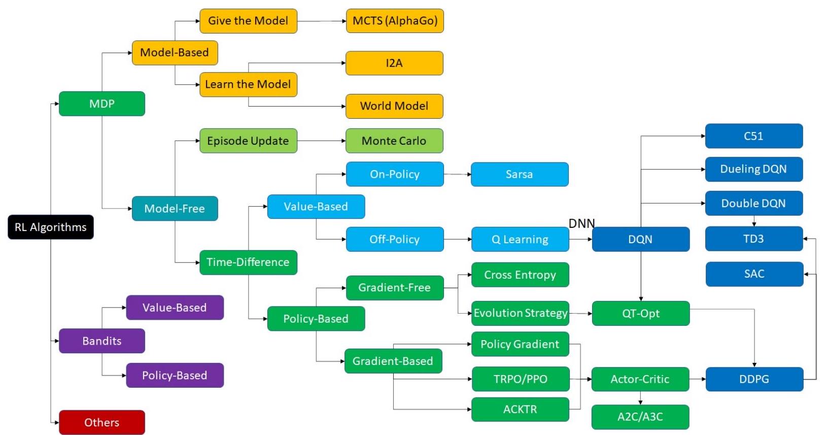
The classification of machine learning algorithms can be complicated and is still evolving quickly due to the fast development of RL. Fig. 15.3 presents a classification that includes the most classic and popular algorithms in the state of the practice. Currently, the RL based on MDP is predominant. Both model-based and model-free RL within this category gained success. However, more research and breakthroughs have been made in the time-difference model-free RL, which can be further categorized into value-based and policy-based algorithms. In more recent studies, both value-based and policy-based algorithms have been integrating deep neural networks to enable impactful deep reinforcement learning [160, 161].
The remaining of this chapter will use value-based RL as an entry for introducing reinforcement learning. We will show how to construct the classic Q learning (or Q-learning)[159] and Sarsa [162], from theories, procedure, to pseudocode. In the next chapter, we will focus on policy-based RL algorithms. A classic gradient-based algorithm, policy gradient, will be presented in detail. Based on that, more information will be provided for other gradient-based policybased RL algorithms.

15.4.2. Q Learning and Sarsa

The essence of Q learning is to use the average value of Q ( s , a ) Q ( s , a ) Q(s,a)Q(s, a)Q(s,a) to estimate Q ( s , a ) Q ( s , a ) Q(s,a)Q(s, a)Q(s,a) : a strategy called time-difference. A much different but easier to understand strategy is to collect all (or a large amount of) the data, e.g., one episode, and then calculate the average. This is the strategy adopted by episode-update methods like Monte Carlo. Therefore, distinct from episode update methods, time-difference methods like Q-learning update the average value, e.g., Q ( s , a ) Q ( s , a ) Q(s,a)Q(s, a)Q(s,a), immediately after a new data point (or sample, e.g., s , a , r s , a , r s,a,rs, a, rs,a,r ) is collected instead of after an episode is finished. The math underlying this time-difference can be derived with the following equation.
Figure 15.3: Overview of popular RL algorithms
u k = 1 K k = 1 K x k (15.23) = 1 K ( x K + k = 1 K 1 x k ) = 1 K [ x K + ( K 1 ) u K ] = u K 1 + 1 K ( x K u K 1 ) u k = 1 K k = 1 K x k (15.23) = 1 K x K + k = 1 K 1 x k = 1 K x K + ( K 1 ) u K = u K 1 + 1 K x K u K 1 {:[u_(k)=(1)/(K)sum_(k=1)^(K)x_(k)],[(15.23)=(1)/(K)(x_(K)+sum_(k=1)^(K-1)x_(k))],[=(1)/(K)[x_(K)+(K-1)u_(K)]],[=u_(K-1)+(1)/(K)(x_(K)-u_(K-1))]:}\begin{align*} u_{k} & =\frac{1}{K} \sum_{k=1}^{K} x_{k} \\ & =\frac{1}{K}\left(x_{K}+\sum_{k=1}^{K-1} x_{k}\right) \tag{15.23}\\ & =\frac{1}{K}\left[x_{K}+(K-1) u_{K}\right] \\ & =u_{K-1}+\frac{1}{K}\left(x_{K}-u_{K-1}\right) \end{align*}uk=1Kk=1Kxk(15.23)=1K(xK+k=1K1xk)=1K[xK+(K1)uK]=uK1+1K(xKuK1)
In the above equation, the average value at the current step u K u K u_(K)u_{K}uK is obtained by adding 1 K ( x K u K 1 ) 1 K x K u K 1 (1)/(K)(x_(K)-u_(K-1))\frac{1}{K}\left(x_{K}-u_{K-1}\right)1K(xKuK1) to the average of the previous step u K 1 1 K u K 1 1 K u_(K-1)*(1)/(K)u_{K-1} \cdot \frac{1}{K}uK11K is the learning rate for a constant number of steps. Then, we can use α α alpha\alphaα, a generalized learning rate, to reformulate the above equation as
(15.24) u k = u K 1 + α ( x K u K 1 ) = ( 1 α ) u K 1 + α x K (15.24) u k = u K 1 + α x K u K 1 = ( 1 α ) u K 1 + α x K {:[(15.24)u_(k)=u_(K-1)+alpha(x_(K)-u_(K-1))],[=(1-alpha)u_(K-1)+alphax_(K)]:}\begin{align*} u_{k} & =u_{K-1}+\alpha\left(x_{K}-u_{K-1}\right) \tag{15.24}\\ & =(1-\alpha) u_{K-1}+\alpha x_{K} \end{align*}(15.24)uk=uK1+α(xKuK1)=(1α)uK1+αxK
Thus, this equation provides one way of understanding the world, i.e., characterized by the average or expected value, by continuously taking more measurements and using such measurements to update the average or approach the expected value.
In Q learning, we want to select the action in the current state that can lead to the highest cumulative rewards. Accordingly, we define Q π ( s , a ) Q π ( s , a ) Q^(pi)(s,a)Q^{\pi}(s, a)Qπ(s,a) as the expected value of first taking action a a aaa in state s s sss and then following the policy π π pi\piπ forever. In Q learning, we are improving our understanding of the environment and, consequently, the policy by updating the Q ( s , a ) Q ( s , a ) Q(s,a)Q(s, a)Q(s,a) values. Using the above equation for updating the expected value, Q ( s , a ) Q ( s , a ) Q(s,a)Q(s, a)Q(s,a) can be updated as follows:
(15.25) Q ( s , a ) = ( 1 α ) Q ( s , a ) + α [ r + γ max a Q ( s , a ) ] (15.25) Q ( s , a ) = ( 1 α ) Q ( s , a ) + α r + γ max a Q s , a {:(15.25)Q(s","a)=(1-alpha)Q(s","a)+alpha[r+gammamax_(a^('))Q(s^('),a^('))]:}\begin{equation*} Q(s, a)=(1-\alpha) Q(s, a)+\alpha\left[r+\gamma \max _{a^{\prime}} Q\left(s^{\prime}, a^{\prime}\right)\right] \tag{15.25} \end{equation*}(15.25)Q(s,a)=(1α)Q(s,a)+α[r+γmaxaQ(s,a)]
where r r rrr is the reward gained as we move from state s s sss to the next state s s s^(')s^{\prime}s after taking action a a aaa, and max a Q ( s , a ) max a Q s , a max_(a^('))Q(s^('),a^('))\max _{a^{\prime}} Q\left(s^{\prime}, a^{\prime}\right)maxaQ(s,a) is the maximum of the Q Q QQQ values of all the actions in the state s . γ max a Q ( s , a ) s . γ max a Q s , a s^(').gammamax_(a^('))Q(s^('),a^('))s^{\prime} . \gamma \max _{a^{\prime}} Q\left(s^{\prime}, a^{\prime}\right)s.γmaxaQ(s,a) represents the experience from previous
learning. For example, max a Q ( s , a ) max a Q s , a max_(a^('))Q(s^('),a^('))\max _{a^{\prime}} Q\left(s^{\prime}, a^{\prime}\right)maxaQ(s,a) can inform the agent in the current state if the agent previously (in an early learning process or episode) gained a high reward in state s s s^(')s^{\prime}s after taking action a a a^(')a^{\prime}a. As can be seen, this equation is the same as the Q update equation (Fig. 15.22) using the Bellman equation, disregarding the difference in symbols.
Q learning is off-policy learning, whereby the agent can learn from the data generated beforehand instead of learning as the agent generates data in an environment. An RL algorithm that is very close to Q learning but with a distinct onpolicy nature is Sarsa. In Sarsa, the learning agent must participate in the learning process as it improves the policy. This is achieved by replacing max a Q ( s , a ) max a Q s , a max_(a^('))Q(s^('),a^('))\max _{a^{\prime}} Q\left(s^{\prime}, a^{\prime}\right)maxaQ(s,a) with Q ( s , a ) Q s , a Q(s^('),a^('))Q\left(s^{\prime}, a^{\prime}\right)Q(s,a). Thus, instead of selecting the action leading to the maximum reward in the next state ( s s s^(')s^{\prime}s part of the Q table is from history only (off the policy) at this moment), the agent in Sarsa first uses the policy derived from Q Q Q\mathbf{Q}Q (still on the same policy, with ϵ ϵ epsilon\epsilonϵ-greedy) to get Q ( s , a ) Q s , a Q(s^('),a^('))Q\left(s^{\prime}, a^{\prime}\right)Q(s,a) (next state) and then use this Q ( s , a ) Q s , a Q(s^('),a^('))Q\left(s^{\prime}, a^{\prime}\right)Q(s,a) to update the Q ( s , a ) Q ( s , a ) Q(s,a)Q(s, a)Q(s,a) in the current state:
(15.26) Q ( s , a ) ( 1 α ) Q ( s , a ) + α [ r + γ Q ( s , a ) ] (15.26) Q ( s , a ) ( 1 α ) Q ( s , a ) + α r + γ Q s , a {:(15.26)Q(s","a)larr(1-alpha)Q(s","a)+alpha[r+gamma Q(s^('),a^('))]:}\begin{equation*} Q(s, a) \leftarrow(1-\alpha) Q(s, a)+\alpha\left[r+\gamma Q\left(s^{\prime}, a^{\prime}\right)\right] \tag{15.26} \end{equation*}(15.26)Q(s,a)(1α)Q(s,a)+α[r+γQ(s,a)]
The detailed procedures for implementing Q learning and Sarsa are exemplified using the following pseudo-code.

Q learning:

Initialize Q ( s , a ) Q ( s , a ) Q(s,a)Q(s, a)Q(s,a) arbitrarily
Repeat for each episode:
Initialize s s sss (e.g., choose a s s sss randomly)
Repeat for each step of the episode:
Select a a aaa from s s sss using a policy derived from Q (e.g., ϵ ϵ epsilon\epsilonϵ-greedy 1 1 ^(1){ }^{1}1 )
Take action a a aaa, and obtain r r rrr and s s s^(')s^{\prime}s based on the environment
Update Q : Q ( s , a ) ( 1 α ) Q ( s , a ) + α [ r + γ max a Q ( s , a ) ] Q : Q ( s , a ) ( 1 α ) Q ( s , a ) + α r + γ max a Q s , a Q:Q(s,a)larr(1-alpha)Q(s,a)+alpha[r+gammamax_(a^('))Q(s^('),a^('))]Q: Q(s, a) \leftarrow(1-\alpha) Q(s, a)+\alpha\left[r+\gamma \max _{a^{\prime}} Q\left(s^{\prime}, a^{\prime}\right)\right]Q:Q(s,a)(1α)Q(s,a)+α[r+γmaxaQ(s,a)]
Update s : s s s : s s s:s larrs^(')s: s \leftarrow s^{\prime}s:ss
Until s s sss is terminal

Sarsa:

Initialize Q ( s , a ) Q ( s , a ) Q(s,a)Q(s, a)Q(s,a) arbitrarily
Repeat for each episode:
Initialize s s sss (e.g., choose a s s sss randomly)
Select a a aaa from s s sss using a policy derived from Q (e.g., ϵ ϵ epsilon\epsilonϵ-greedy)
Repeat for each step of the episode:
Take action a a aaa, and obtain r r rrr and s s s^(')s^{\prime}s based on the environment
Select a a a^(')a^{\prime}a from s s s^(')s^{\prime}s using a policy derived from Q (e.g., ϵ ϵ epsilon\epsilonϵ-greedy
Update Q : Q ( s , a ) ( 1 α ) Q ( s , a ) + α [ r + γ Q ( s , a ) ] Q : Q ( s , a ) ( 1 α ) Q ( s , a ) + α r + γ Q s , a Q:Q(s,a)larr(1-alpha)Q(s,a)+alpha[r+gamma Q(s^('),a^('))]Q: Q(s, a) \leftarrow(1-\alpha) Q(s, a)+\alpha\left[r+\gamma Q\left(s^{\prime}, a^{\prime}\right)\right]Q:Q(s,a)(1α)Q(s,a)+α[r+γQ(s,a)]
Update s : s s s : s s s:s larrs^(')s: s \leftarrow s^{\prime}s:ss
Until s s sss is terminal
Example code for implementing Q learning to address the Taxi-v3 problem is given in the following.
import numpy as np
              import pandas as pd
              import gym
              # Initialization
              env = gym.make("Taxi-v3") # Call the "Taxi-v3" environment from gym with the name "env"
              action_size = env.action_space.n # Obtain the size of the action space: how many actions. There are
                six here
              state_size = env.observation_space.n # Obtain the size of the state space: 5 rows * 5 columns * 5
                passenger positions * 4 destinations =500 states
              Table = np.zeros((state_size, action_size)) # Initialize the Q table
              # Hyperparameter
              epsilon = 0.9 # Parameter for epsilon-greedy
              alpha = 0.1 # Learning rate
              gamma =0.8 # Decay of rewards
              # Training
              n_episode = 10000 # Number of episodes for training
              
for n in range(n_episode):
                state = env.reset() # Initialize the environment for each episode
                while True:
                    # Choose an action based on the Q table with epsilon greedy
                    action_Q = np.argmax(Table[state]) # Choose an action based on the Q table
                    action_greedy = np.random.choice(Table[state].size) # Choose an action randomly for use in
                the epsilon-greedy method
                    action = np.random.choice([action_Q,action_greedy],size=1,p=[epsilon,1-epsilon])[0]
                    # Update state
                    state_new, reward, done, _ = env.step(action)
                    # Update the table
                    Table[state,action] = (1-alpha)*Table[state,action] + alpha*(reward+gamma*max(Table[
                state_new]))
                    # Prepare for the next step
                    state = state_new
                    # Stop an episode when the environment tells an episode ends
                    if done == 1:
                        print('This is the %i the episode' % n)
                        break
              # Testing
              state = env.reset()
              while True:
                # Choose an action based on the Q table only
                action = np.argmax(Table[state]) # Choose action based on Q table
                state, reward, done, _ = env.step(action)
                env.render() # Green is passenger; Red is destination
                if done == 1:
                    break
              

15.4.3. Monte Carlo Method

In the current practices of reinforcement learning, the use of episodic update methods represented by the Monte Carlo method is less popular than step-update method (time-difference) methods. Compared to time-difference methods such as Q learning and Sarsa, the Monte Carlo method is also value-based: the learning is carried out by improving the value functions. However, instead of updating the value functions step by step in an episode, the Monte Carlo method first finishes all the steps in the episode and then updates the value. Accordingly, for each episode, a series of states will be generated randomly: s 1 , a 1 , r 2 , s 2 , a 2 , r 3 , , s t , a t , r t + 1 , , s T , a T s 1 , a 1 , r 2 , s 2 , a 2 , r 3 , , s t , a t , r t + 1 , , s T , a T s_(1),a_(1),r_(2),s_(2),a_(2),r_(3),cdots,s_(t),a_(t),r_(t+1),cdots,s_(T),a_(T)s_{1}, a_{1}, r_{2}, s_{2}, a_{2}, r_{3}, \cdots, s_{t}, a_{t}, r_{t+1}, \cdots, s_{T}, a_{T}s1,a1,r2,s2,a2,r3,,st,at,rt+1,,sT,aT.
Then let us recall the definition of the value function in the MDP. However, a minor difference is made so that the equation can be used to calculate the value of every state in a series of states.
(15.27) V π ( s ) = E π ( G t s t = s ) = E π [ i = t T γ i t r i + 1 ] (15.27) V π ( s ) = E π G t s t = s = E π i = t T γ i t r i + 1 {:(15.27)V^(pi)(s)=E^(pi)(G_(t)∣s_(t)=s)=E^(pi)[sum_(i=t)^(T)gamma^(i-t)r_(i+1)]:}\begin{equation*} V^{\pi}(s)=\mathbb{E}^{\pi}\left(G_{t} \mid s_{t}=s\right)=\mathbb{E}^{\pi}\left[\sum_{i=t}^{T} \gamma^{i-t} r_{i+1}\right] \tag{15.27} \end{equation*}(15.27)Vπ(s)=Eπ(Gtst=s)=Eπ[i=tTγitri+1]
Therefore, for every step in an episode, we will have one state s s sss (and choose one action a a aaa ), which corresponds to a G t G t G_(t)G_{t}Gt value in the above function. Using the average value update equation, we can update the value function of every state s s sss that appears in a series (episode):
(15.28) V ( s ) = ( 1 α ) Q ( s ) + 1 N G t (15.28) V ( s ) = ( 1 α ) Q ( s ) + 1 N G t {:(15.28)V(s)=(1-alpha)Q(s)+(1)/(N)G_(t):}\begin{equation*} V(s)=(1-\alpha) Q(s)+\frac{1}{N} G_{t} \tag{15.28} \end{equation*}(15.28)V(s)=(1α)Q(s)+1NGt
where N N NNN is the number of times that this state appears in the whole learning process (e.g., all the episodes that have been tested). It is possible that a state can appear multiple times in an episode (series). To deal with such a situation, we can choose to consider only the reward gained ( G t ) G t (G_(t))\left(G_{t}\right)(Gt) in the first appearance of this state (called first visit) or use the rewards from every appearance of the state (called every visit). The second method usually requires more computational effort but may get better results when the number of series is small.
In fact, we usually update the action-value function ( Q table). This update can be performed in a similar way:
(15.29) Q ( s , a ) = ( 1 α ) Q ( s , a ) + 1 N G t (15.29) Q ( s , a ) = ( 1 α ) Q ( s , a ) + 1 N G t {:(15.29)Q(s","a)=(1-alpha)Q(s","a)+(1)/(N)G_(t):}\begin{equation*} Q(s, a)=(1-\alpha) Q(s, a)+\frac{1}{N} G_{t} \tag{15.29} \end{equation*}(15.29)Q(s,a)=(1α)Q(s,a)+1NGt
To use the equation, we need to record the N N NNN number for every state for updating the state value and for every action in every state for updating the action-state value. This will consume a lot of memory. A convenient alternative is to replace 1 N 1 N (1)/(N)\frac{1}{N}1N with a learning rate α α alpha\alphaα.

  1. 1 1 ^(1){ }^{1}1 Select a a aaa that has the highest Q Q QQQ at the s s sss with probability of ϵ ϵ epsilon\epsilonϵ and select a random action with a probability of 1 ϵ 1 ϵ 1-epsilon1-\epsilon1ϵ


Enjoy and Build the AI World

Sample Code from AI Engineering

Cite the code in your publications

Linear Models